


Introduction
AI model predictions are increasingly affecting everyone’s lives: search results, purchasing recommendations, loan assessments, and resume screening during recruitment, are just some examples. To ensure that these automatic systems behave appropriately and don’t cause damage, it’s necessary to explain what constitutes the AI’s prediction. For example, which words from the input were important in making the prediction? There have been many approaches to answering this question. However, it has previously been found that none of them work consistently [1]. Even getting to that conclusion is tremendously tricky as we don’t actually know what a true explanation looks like.
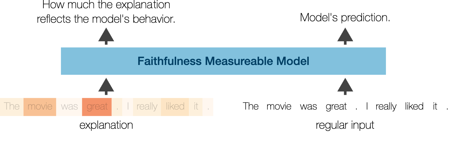
In this work, we propose a new direction in the field: to develop models with a built-in mechanism for telling if an explanation is true, so-called Faithfulness Measurable Models. Because this mechanism is built-in, it’s very cheap to compute and produce accurate results. This also enables us to find the optimal explanation given a prediction, something previously impossible. The result is that explanations consistently reflect how the model behaves and are 2x-5x more accurate than previously.
Faithfulness Measurable Models
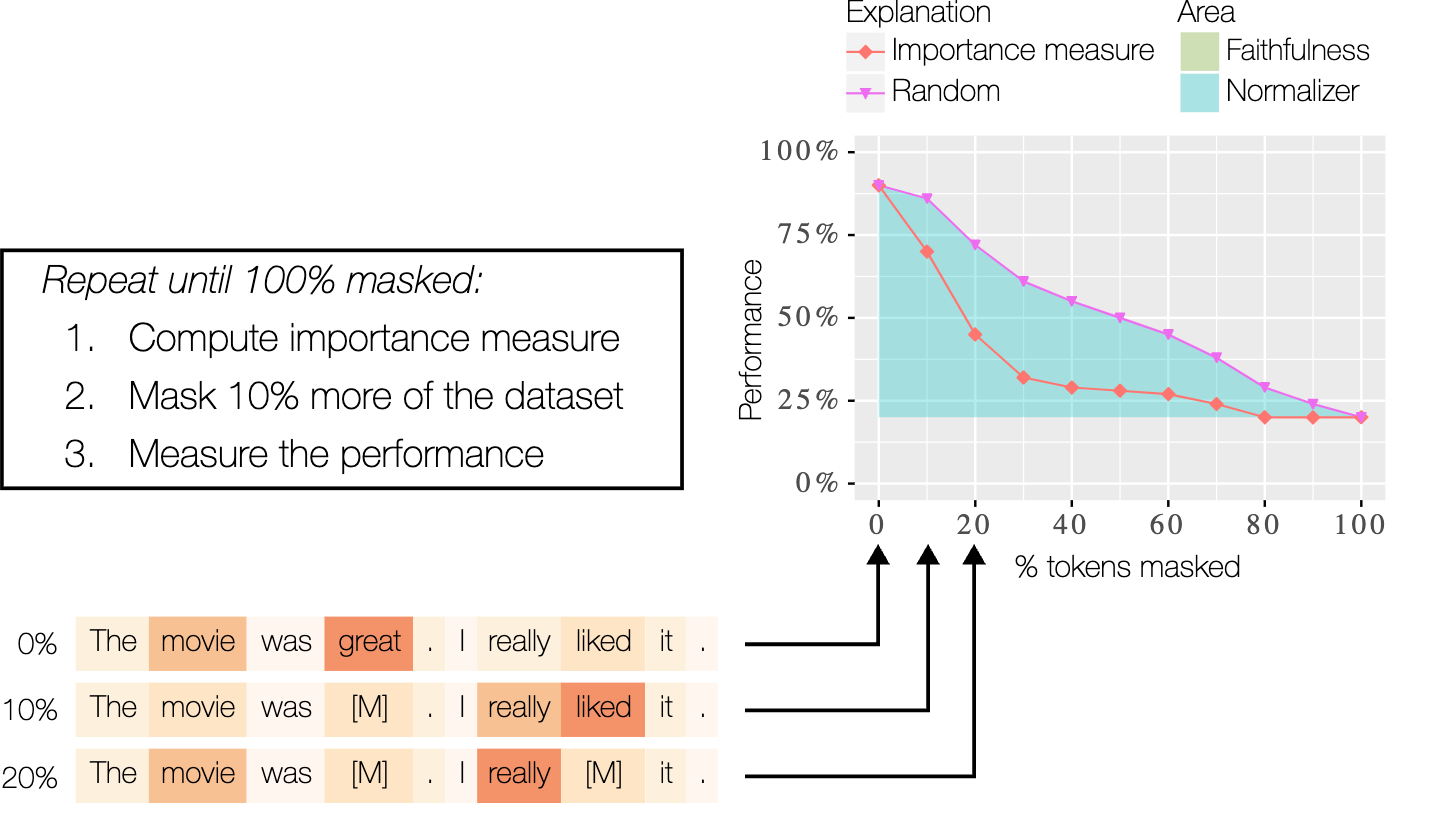
The central idea for identifying whether an explanation reflects the model is that if allegedly important words are removed, the model’s prediction should change a lot, specifically more than if random words are removed. In the context of text, removal is often done by replacing it with a special mask token.
Unfortunately, it’s not possible to just mask words, as this creates ungrammatical inputs, which a typical model is not able to work with. Previous works have solved this by retraining the model, on the partially masked datasets [1]. However, this is expensive to do, as the model has to be retrained 10 times for each dataset and explanation being analyzed. Additionally, it means that we are stepping away from the model that is in deployment because we are now measuring on a different model. This makes this retraining method both difficult to apply and potentially dangerous, as it can lead to false confidence in an explanation.
This leaves us in-between a rock and a hard place. On one side, if the model does not support removal/masking this creates a false measurement. And if we retrain the model to support removal/masking, it also creates a false measurement. The solution to this is to ask: what if we had just one model that supported removal/masking to begin with?
Such a model is the central idea in this paper and is surprisingly easy to achieve. It is done by masking half of the training dataset randomly, with a masking ratio between 0% and 100%. As such, the model learns to both do normal predictions but also predictions where input has been masked. We call this idea “masked fine-tuning” and visualize it in Figure 2.
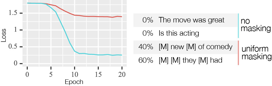
To verify this works, both in terms of not affecting the regular performance and supporting masking, we perform a number of tests. First, we show that no performance is lost using masked fine-tuning compared to using regular (plain) fine-tuning where no masking is done. We show this across 16 common natural language processing datasets. Secondly, as a simple test for masking support we replace all words with the special mask token. At 100% masking we know essentially nothing about the input, so the best the model can do is to predict the class that appears the most often (termed class-majority baseline). We show that only when masking is used, do models’ performance match this baseline.
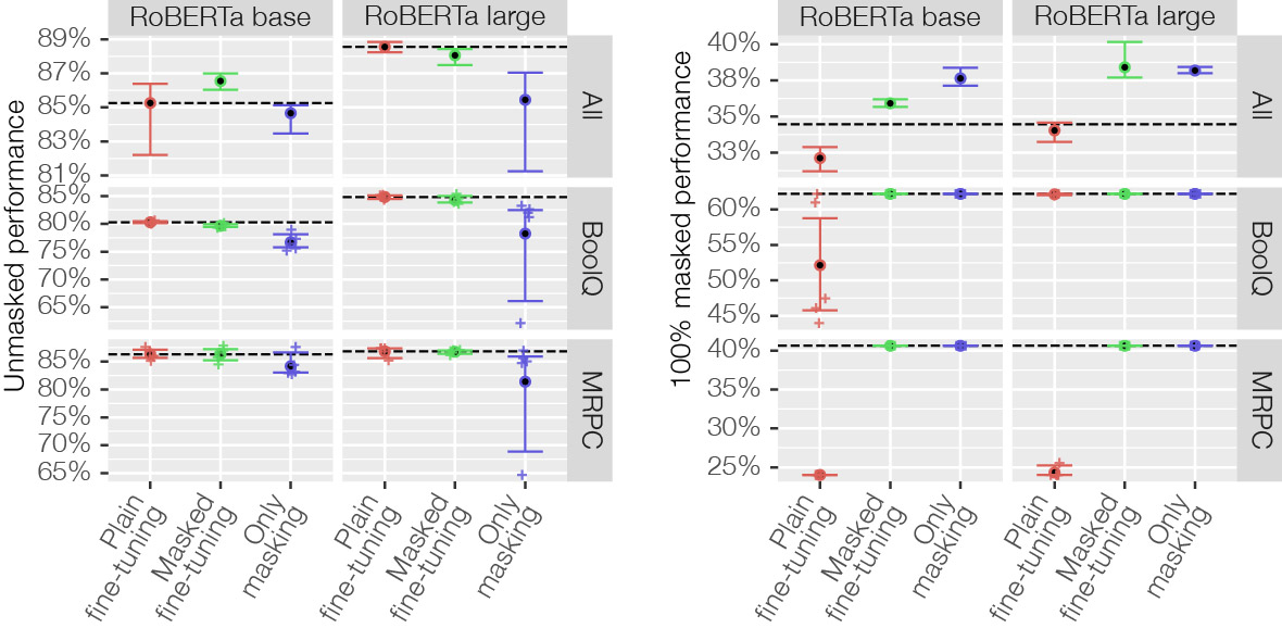
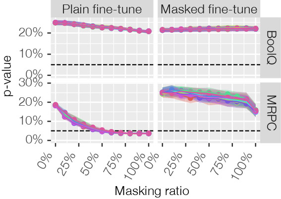
The results in Figure 3, confirm that the model works for 0% masked inputs and 100% masked inputs. However, what about everything in between? For these levels of masking we do not know what performance to expect. To solve this, we perform a statistical test to check if the model behaves as it would normally behave. The test we apply is called MaSF [2], the details of which are too complicated to cover in this blogpost, however the gist of it is to observe the model’s intermediate activations for the validation dataset and then see if the activations given a new observation is within that activation span. But suffice to say, the results in Figure 4 shows that when applying masked fine-tuning there are never any issues, while when applying the ordinary plain fine-tuning some datasets present issues where the model breaks.
Now that we know the model behaves as desired, we can measure if the explanations reflect the model. As a reminder, the central idea is that if important words are removed, the model’s prediction should change a lot, specifically more than if random words are removed. From the results in Figure 5, it’s clear that Leave-one-out (LLO) and Beam [3] are the best performing. This makes sense as they take advantage of the masking support, while the other explanation methods do not. Beam in particular is interesting, as this identifies the explanation that reflects the model’s behavior as much as possible using an optimization method. This is possible because the Faithfulness Measurable Model makes determining this cheap and efficient. The details [3] are not important for this blog post, but the gist is to consider each word as the most important word, measure how good each of these explanations are, and then select the top 3 best explanations (or choose any number). Then for these 3 explanations, the second most important word is identified and so on, always keeping the best 3 candidate explanations until the best ranking of word importance of all words is identified. Because only the top 3 explanations are considered, this is an approximate method, so it’s not always the best but it frequently is.
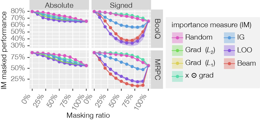
How much the explanation curve is below the random curve can also be quantified by computing the area-between-curves. For absolute explanations, which are those that cannot separate between positive and negative contributing words, this can then be normalized by what is the theoretical optimal explanation, as shown in Figure 1. This makes it easy to compare with other methods and models, in this case we compare with Recursive ROAR which uses retraining [1].
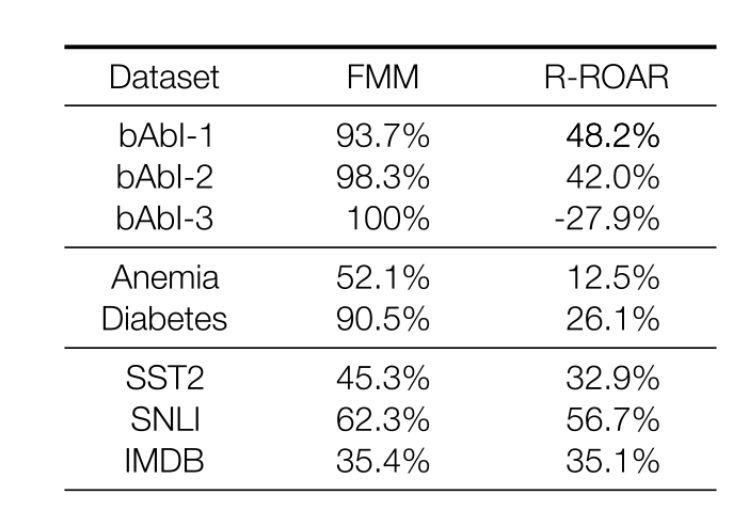
The result of this comparison can be seen in Table 1. Here we observe often between 2x and 5x improvement. However, more importantly we observed that there exists explanations that consistently reflect the model behavior, which has not previously been the case and that for synthetic datasets like (bAbI) the explanations are close to theoretical perfection.
Conclusion
Using a simple modification to how models are usually fine-tuned, we are able to create a model where it’s possible to cheaply and accurately measure how much an explanation reflects the model’s true behavior, which enables optimizing explanations towards maximal truth. We call such a model a Faithfulness Measurable model.
In addition to this we find that existing explanations consistently reflect how the model behaves, are 2x-5x more accurate, and can operate with near theoretical perfection. Finally, the modified fine-tuning procedure doesn’t cause any performance impact, which we verify on 16 datasets.
References
[1] Madsen, A., Meade, N., Adlakha, V., & Reddy, S. (2022). Evaluating the Faithfulness of Importance Measures in NLP by Recursively Masking Allegedly Important Tokens and Retraining. Findings of the Association for Computational Linguistics: EMNLP 2022, 1731–1751. https://aclanthology.org/2022.findings-emnlp.125
[2] Matan, H., Frostig, T., Heller, R., & Soudry, D. (2022). A Statistical Framework for Efficient Out of Distribution Detection in Deep Neural Networks. International Conference on Learning Representations. https://openreview.net/forum?id=Oy9WeuZD51
[3] Zhou, Y., & Shah, J. (2023). The Solvability of Interpretability Evaluation Metrics. Findings of the Association for Computational Linguistics: EACL. http://arxiv.org/abs/2205.08696