


Heating, Ventilation and Air Conditioning systems: a key of the energy transition.
Buildings account for one third of the energy consumption worldwide, half of which is used by Heating Ventilation and Air Conditioning (HVAC) systems. These systems are responsible for 15% of the CO2 emissions. Optimally controlling these systems is crucial for conserving energy and reducing the impact of climate change.
The energy demand varies throughout the day, depending on the weather and consumers’ habits. Peak periods, when the energy demand is the highest, are particularly challenging for grid operators and often coincide with periods where HVAC systems use the most energy. In many countries such as Canada, the United States or France, Demand Side management measures are developed to encourage consumers to limit their energy usage, especially during peak periods. One of these strategies, called Demand Response (DR) programs, consists in changing the electricity price to give incentives to consumers to reduce their peak power usage.
Among the various loads that can be managed to influence power usage, HVAC systems are particularly important due to their significant share of total power consumption. Additionally, optimizing HVAC systems does not directly affect occupant comfort because of the thermal inertia of buildings. Similar to a battery, a building can store heat, enabling pre-heating or pre-cooling strategies to proactively reduce power usage during peak times.
To manage HVAC power usage, indoor temperature set points can be adjusted. To address demand response events while accounting for exogenous perturbations such as occupants and weather, a building model is needed to predict the impact of set point changes on indoor temperature and power consumption. These models can be based on the building’s blueprint, but this approach is often time-consuming and limits large-scale implementation. Alternatively, models can be developed using metered temperature and power data. While this approach is more systematic, it often requires substantial data for accurate predictions, hindering widespread adoption.
The novelty of our approach
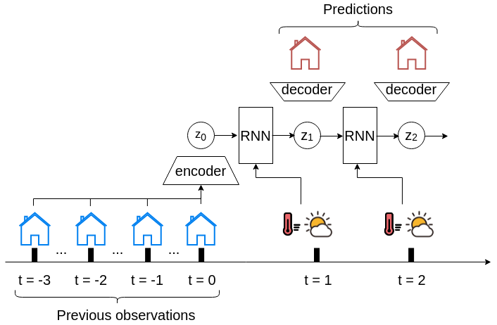
Data-driven models are frequently employed to make predictions in a discrete time setting, where the mode forecasts the system’s state at the next time step Zt+1 based on the current state Zt and upcoming actions and weather forecast. A building is a partially observable system, and state observation lags are encoded in a latent space used for making predictions. These models are called State Space Models (SSM), and implemented with a Recurrent Neural Network (RNN) and an encoder/decoder structure, as depicted below.
In our work, we propose a continuous-time formulation to the prediction task and use Neural Ordinary Differential Equations (NODE) to model the building’s dynamics. Unlike the discrete-time SSM presented above, continuous-time models do not learn a function f to predict the next state from the previous state as : \[Z_{t+1} = f\,_0(z_t)\].
Instead, a function g, often called the vector field, is learned to represent the continuous evolution of the state with time. This function can be thought of as the derivative of the state, describing the state changes. To compute future state values, one needs to integrate the vector field from an initial state: ![]()
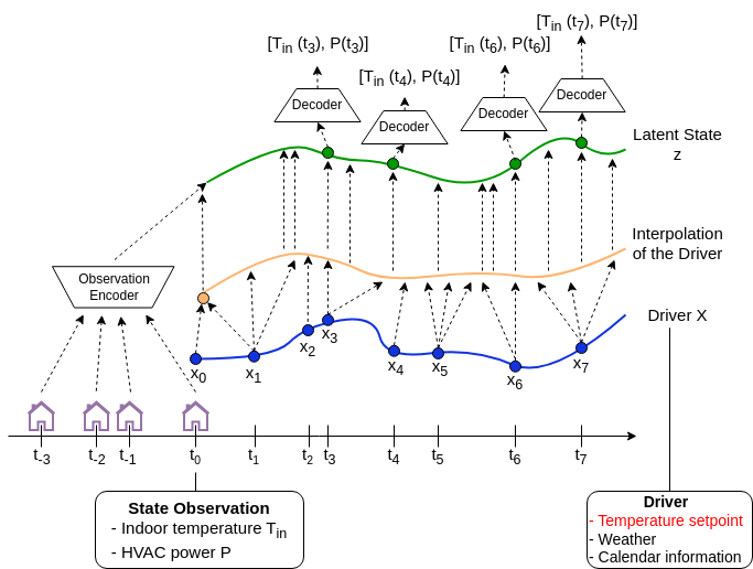
Such models may be seen as the continuous counterparts of Residual Networks or RNN. To account for future actions or weather forecast, one can parametrized the vector field as g(zt; xt), where Xt is the driver value at time t. As illustrated below, the upcoming actions and disturbances are interpolated in a continuous signal used to compute the state’s evolution.
The idea of using a continuous-time framework is that the underlying process we are trying to model, i.e. the evolution of the temperature in a building, is continuous. It is therefore advantageous to use a continuous model.
One of the weaknesses of fully data-driven models is that the resulting model is not guaranteed to respect the law of physics. Physics informed, or structured, models have been developed to enforce physics constraints to data-driven models. We thus propose NODE models encoding the law of energy conservation to make our models realistic. These models are referred to as “structured” models in the following.
Finally, one advantage of continuous-time models is that they are better suited to handle irregular and missing data. For planning purposes, handling irregular and missing data is mostly relevant in the encoder part, as there is no purpose in making irregular predictions to plan for indoor temperature setpoints. We thus propose continuous-encoders (CE) to build more informative latent states.
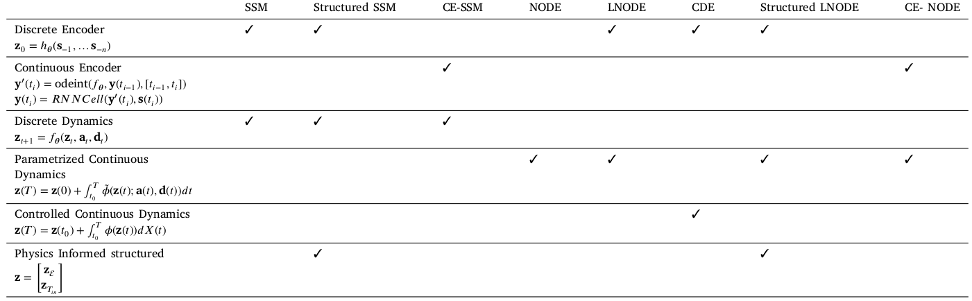
Continuous-time (NODE) models including physics-informed structure and continuous-time and discrete-time encoders and are all compared to their discrete counterparts (the SSM models). The table below gives an overview of the tested models.
The purpose of prediction models is to inform decisions. We thus embed the prediction model in a Model Predictive Control (MPC). We formulate the control problem with a hard constraint on the maximum power usage to prioritize energy savings over comfort at peak time. We also use comfort temperature intervals instead of fixed setpoints to enhance energy conservation while maintaining a minimum level of comfort for the occupants.
Experimental results
To assess the performances of NODE models, we first compare their prediction accuracy with their discrete-time counterpart of simulated and real-world data. Our key finding is that continuous-time models require less training data than discrete-time models.
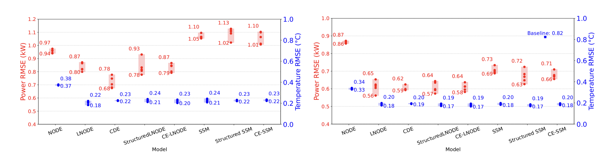
The graphs below show the Root Mean Square Error (RMSE) on 2h and ahead predictions of the temperature and HVAC power for a house modeled in EnergyPlus. The models are trained with 2.5 months of training data (left figure) and 10 months of training data (right figure). The five models positioned furthest to the left are continuous-time models, while the three on the right are discrete-time models. One can observe the better performances of the continuous-time model, especially when trained with fewer data.
Regarding the control, both continuous-time and discrete-time models obtain similar control performances when used with MPC to lower the power consumption during peak hours. The graph below is a four day example of control using the LNODE (continuous-time) model during winter. The red curve represents the HVAC power consumption of the house, and the yellow curve represents the power consumption without MPC. The blue curve is the power consumption predicted by the model, on which the control actions are planned.
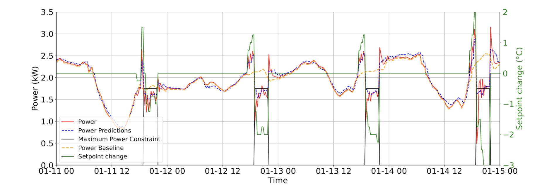
We observe that our control system is able to find pre-heating strategies, increasing the temperature setpoint before the peak period to store heat before lowering the power consumption at peak time. We also notice the importance of prediction accuracy to handle maximum power constraints. For instance, on the second day displayed, the predicted power consumption stays below the maximum whereas during one timestep the real power consumption exceeds the maximum. Giving slack to the maximum power constraint is a simple and efficient way to mitigate the prediction errors.
Conclusion
In this work, we propose novel data-driven continuous-time models to forecast the indoor temperature and HVAC power consumption in buildings. Our empirical results show that continuous-time models are more sample-efficient than their discrete counterparts, that are currently widely used in practice. In addition, we propose a MPC algorithm to use the prediction models to plan for the optimal indoor temperature setpoints during peak-demand periods. Our results show that both continuous and discrete-time models may effectively be used for planning to reduce power consumption while preserving user comfort.