

Generative flow networks (GFlowNets) are new machine learning algorithms for learning to sample from distributions over compositional objects. These distributions are often complicated, e.g., they might have many peaks or modes and are thus challenging to sample from. GFlowNets address this challenge by leveraging advances from deep learning. They have been successfully applied to drug discovery, the modeling of causal graphs, and other domains. By modeling the full distribution over plausible solutions, these new algorithms can lead to more capable AI systems that can aid complex design scenarios, accelerate scientific discovery, and reason robustly like we do.
For a tutorial on GFlowNets, check out https://tinyurl.com/gflownet-tutorial.
GFlowNets are closely related to many existing AI research areas, including reinforcement learning and variational inference. Reinforcement learning (RL) models the behavior of agents who seek to maximize the expected reward through their interaction with an environment. Variational inference (VI) turns the problem of inference into that of approximating intractable probability distributions. GFlowNets solve a variational inference problem using reinforcement learning methods. Let’s take drug discovery as an example. We have a reward model that judges the drug-worthiness of a given molecule. It is tempting to ask for the molecule that maximizes the reward, but since the model only approximates the drug-worthiness, we want to have multiple candidates under the model to test out in the real world. Therefore, we would like to approximately sample molecules proportional to their worthiness under the model, which is a VI problem. Similar to RL, a GFlowNet would break down the generation of a molecule into a sequence of simple actions, such as adding an atom. By minimizing the GFlowNet objectives to zero, we will have obtained such a sampler at the end of training.
In our work, we elucidate the connection between GFlowNets and Variational Inference.
Variational methods, originally a tool in mathematical physics, have led to several of the most important ideas in machine learning over the last few decades, including wake-sleep algorithms and variational auto-encoders (VAEs). The key idea behind VI can be described as “inference via optimization.” Given an intractable distribution to sample from, instead of directly sampling from it, we ask “what is a simple distribution we know how to sample from that approximates the true distribution?” The simple distribution we choose often has trainable parameters, such as the mean and covariance of a Gaussian distribution. By optimizing these parameters, we are able to approximate the true distribution while drawing samples with relative ease.
At first glance, GFlowNets and VI solve different problems. For example, VI is typically applied to continuous random variables, whereas GFlowNets model complex discrete structures constructed in many steps. Some VI algorithms, such as hierarchical and nested VI, are applicable to this setting, in which the target distribution is approximated by sampling a sequence of random quantities one at a time, each choice depending on the previous ones. However, these algorithms use different optimization objectives: VI minimizes divergence metrics between sampled and target distributions, while GFlowNets optimize objectives like flow matching or trajectory balance, which not only fit the target distribution but also optimize measures of internal consistency. In our paper, GFlowNets and Variational Inference, we present a unified view of these two frameworks and study their respective tradeoffs.
In short, GFlowNets with the trajectory balance objective is closely related to hierarchical VI. However, the hierarchical VI objective tends to model only the best solution (using reverse KL divergence) or a blend of many solutions (using forward KL divergence). The GFlowNet objectives offer a better tradeoff between the two and find more high-quality modes. Furthermore, GFlowNet objectives yield a more stable gradient and can be made more powerful by training off-policy. A policy is a decision-making model that tells us what to do in any given situation. For example, given a partially constructed molecule, a policy tells us which atom to add next to build a good drug candidate in the end. Off-policy learning improves a policy by following a different, potentially more exploratory, policy, which helps to capture diverse solutions under the reward function. Imagine we know a few ways to construct good drug molecules. If we stick with what we know, meaning always generating on-policy, we never get a chance to explore more effective combinations of atoms than what we already know; off-policy learning allows us to take a chance and potentially learn something new. Our experiments show that GFlowNets are much easier to learn off-policy compared to hierarchical VI. This is because the GFlowNet objectives do not require importance sampling while hierarchical VI does.
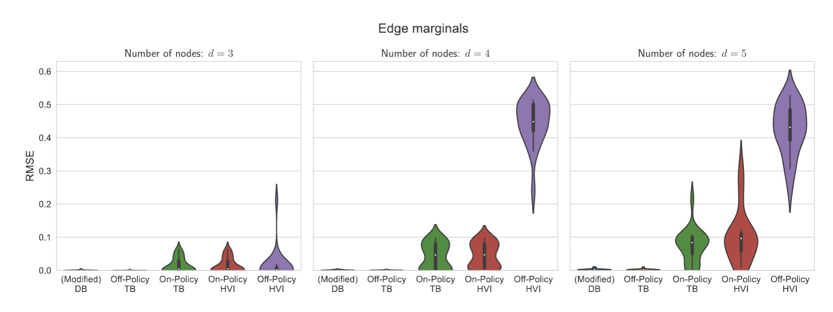
In one of our empirical experiments, we study how well GFlowNets and hierarchical VI can model a distribution over causal graphs given observational data. Causal graphs model the causal relationships among variables of interest. For example, both ice cream consumption and temperature correlate with a crowded beach. However, only one such relationship is causal. In general, due to the lack of interventional data, there are many causal graphs that could fit the data while there is only one true model. This ambiguity makes it important to capture all likely modes instead of committing to any single one.
When there are multiple good solutions or modes, we call the corresponding distribution over solutions multimodal. The distribution over graphs in the example above is multimodal because many graphs are equally capable of explaining the observations. Furthermore, this particular distribution has a complexity that grows exponentially in the size of the graph. Consequently, we observe a significant advantage to using GFlowNets even on small graphs. On graphs with only three nodes, the mean performance is nearly identical for both GFlowNets and hierarchical VI as measured by RMSE (lower is better). However, as the size of the graphs increases to four and five, off-policy learning becomes necessary and GFlowNets drastically outperform HVI.
We hope future works can discover better GFlowNet training methods based on existing literature on hierarchical VI and vice versa. For more details, please check out our paper on arXiv https://arxiv.org/abs/2210.00580.