

Introduction
The world around us is 3-dimensional, yet vision, one of the most important ways that we observe the world, relies heavily on 2-dimensional representations. This is true of both biological vision and computer vision. For this reason, many of the seminal moments in machine learning and deep learning history involve 2D image data. The use of deep convolutional neural networks to achieve record breaking performance in the 2012 ImageNet challenge brought widespread attention to the field of deep learning. More recently, generative image and video models, such as DALL-E and Sora by OpenAI, have had a significant cultural impact.
In the coming years, thanks to developments in the field of differentiable visual computing (DVC), many groundbreaking machine learning technologies will make the jump from 2D to 3D. These innovations will impact sectors involving 3D object detection and scene understanding, computational art and design, manufacturing, autonomous vehicles, robotics, optimal control, and physical inference. These are all sectors in which physically accurate and interpretable models are important, and in which black-box deep learning approaches may not be suitable. DVC allows humans to insert scientific knowledge into a deep learning pipeline, making models more data efficient and more easily interpretable and controllable. Already, these techniques have been applied to design products with special optical properties, to control soft body robots, to capture basketball stars in 3D, to infer object properties like mass and elasticity from video, and much more.
The Differentiable Graphics Pipeline
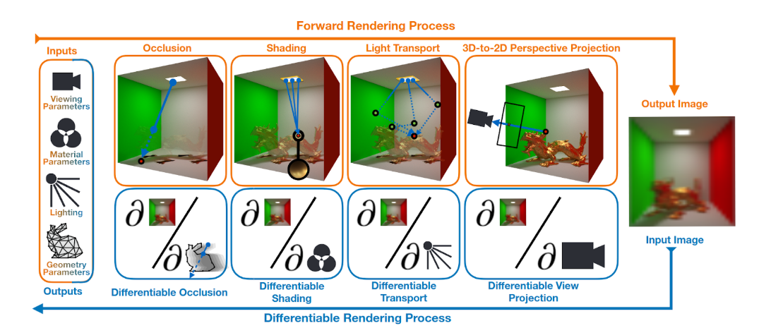
Visual computing (VC) methods can create realistic 2D images of virtual 3D worlds using algorithms to simulate physical processes such as light transport, and the dynamics of fluids, rigid-bodies and other media. The process of turning 3D virtual worlds into 2D images or videos can be considered the “forward” direction of a physical simulation. In some applications, we are also interested in learning information about the 3D world from 2D data. This complementary process is called an “inverse” problem. Solving inverse problems allows us to learn and design virtual 3D worlds in order to produce a particular outcome or effect in a physical simulation or visual computing pipeline.
To solve an inverse problem, we must efficiently search the high-dimensional space of parameters describing a 3D scene in order to find an optimal set of parameters. These parameters could represent the geometry of an object, the optical properties of an object (e.g. color, reflectivity, or translucency), the physical properties of an object (e.g. mass, viscosity, or elasticity), or the properties of an imaging system (e.g. the camera position, orientation, or focal depth). In deep learning, such parameter searches are typically conducted using gradient-based optimization algorithms. This approach, however, is predicated on the property of differentiability with respect to a set of parameters. Thus enters the field of differentiable visual computing (DVC). By designing visual computing and graphics pipelines that support differentiation, we can utilize the same optimization approaches that are used to train deep learning models. Furthermore, DVC components can seamlessly integrate with deep learning models to create hybrid systems consisting of flexible deep learning models and physically accurate simulations.
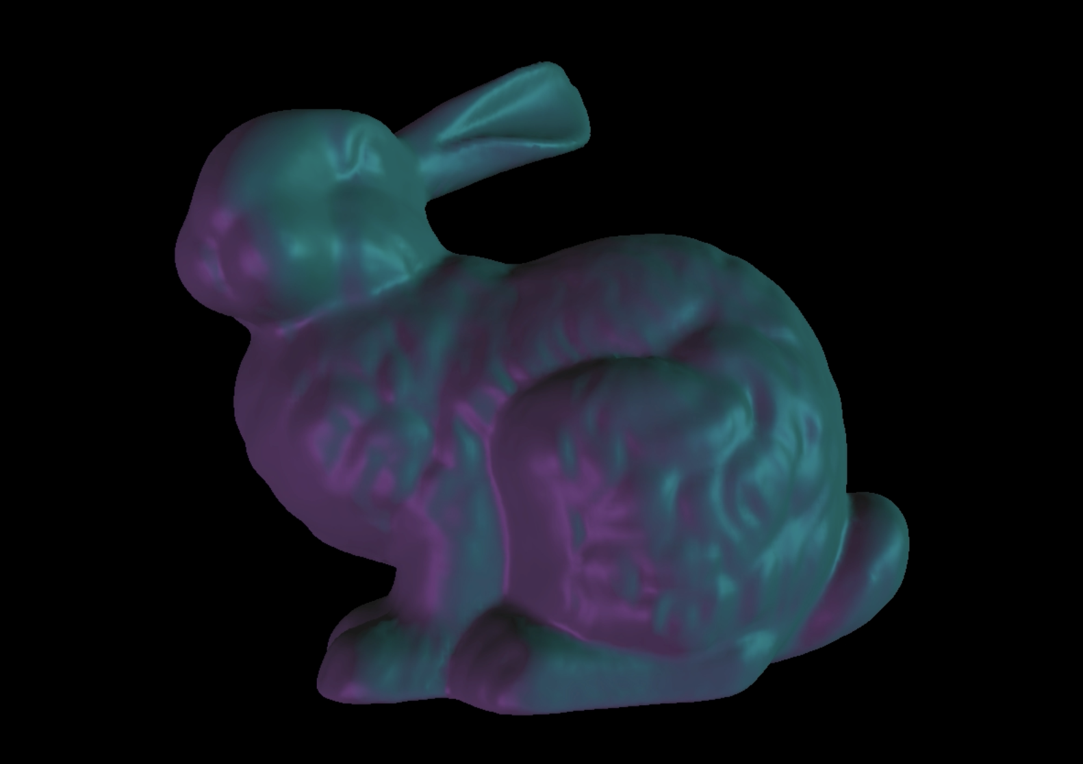
One of the core components of a differentiable graphics pipeline is a differentiable renderer. Just like regular renderers, differentiable renderers can run a forward rendering process, in which a 3D scene is turned into a realistic 2D image. Additionally, differentiable renderers can backpropagate gradients from a rendered image to the 3D scene parameters. This allows for applications where 3D scene parameters are learned from 2D image supervision. Video 1 shows an example where the lights illuminating a bunny mesh are learned using gradient descent optimization and a ground truth image of the bunny. The 3D bunny model was obtained from The Stanford 3D Scanning Repository.
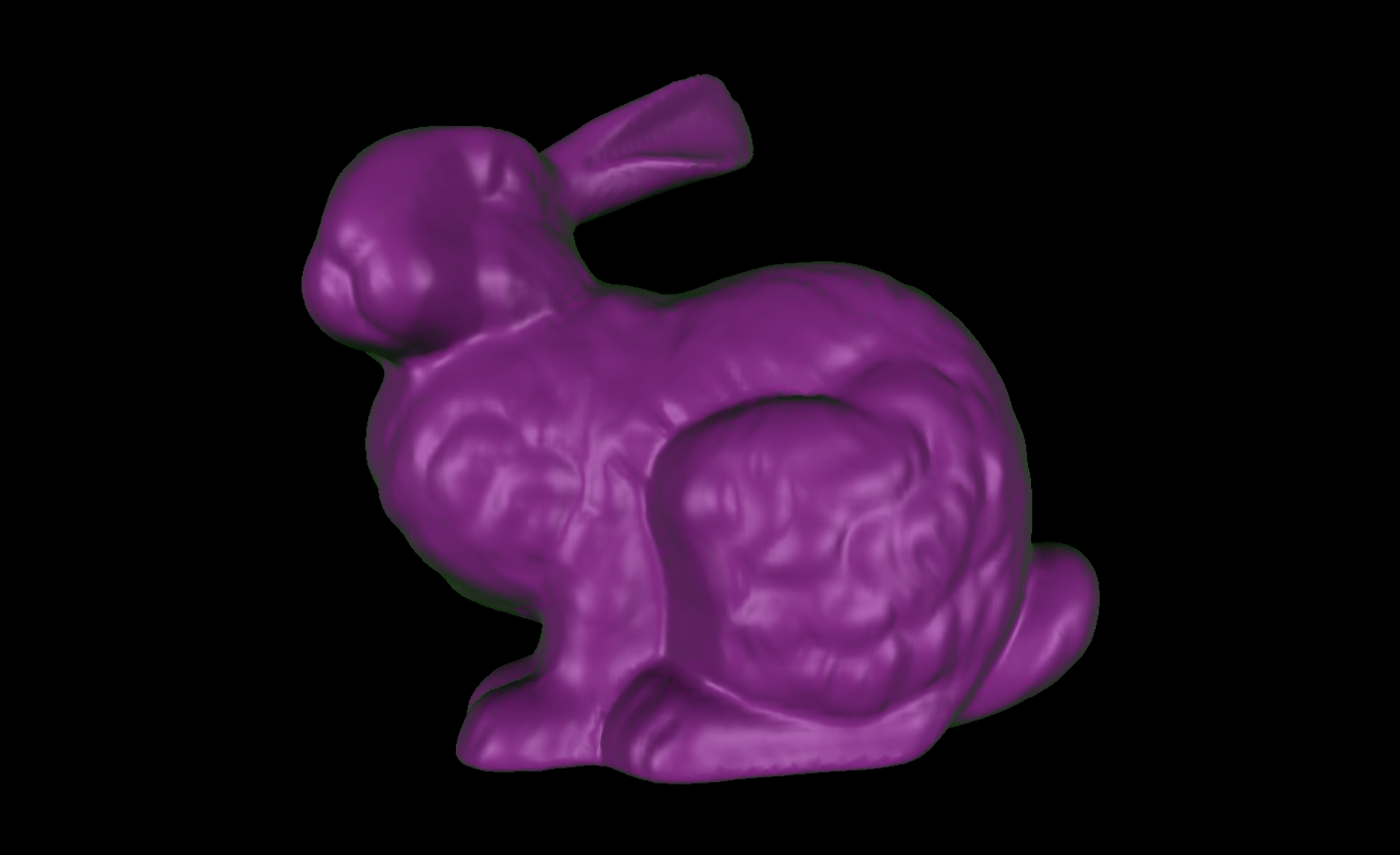
Video 2 shows an example where the material of a bunny mesh is learned using gradient descent optimization and a ground truth image of the bunny.
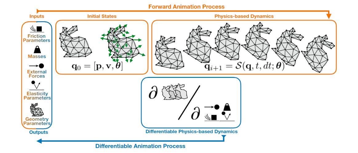
Frequently, VC pipelines are used to create images of dynamic 3D scenes. In such scenes, objects may be animated (e.g. character body movements), or their dynamics may be generated using physical simulations (e.g. the movement of clothing or hair in response to character body movement). These simulations can also be made differentiable and integrated into a DVC pipeline. This allows for applications where physical parameters (e.g. object mass, elasticity, or external forces) or animations are learned from 2D or 3D data.
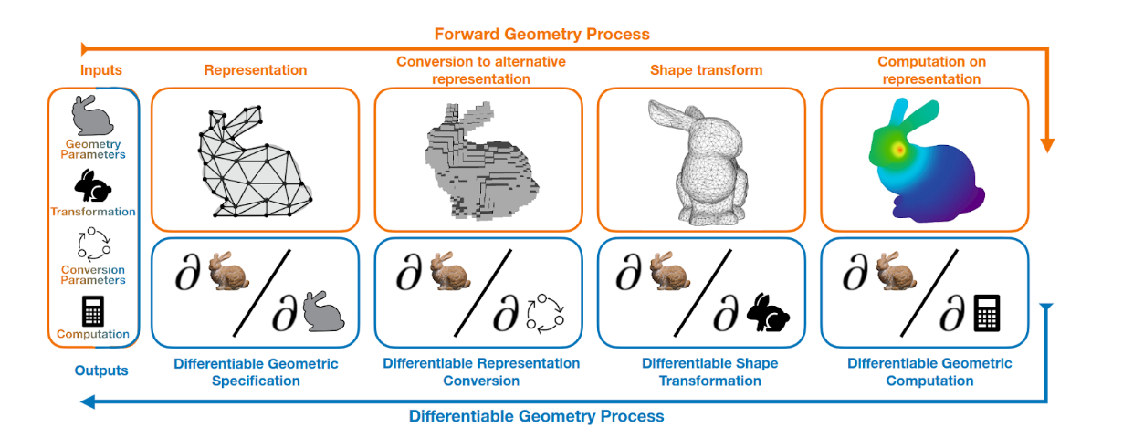
In different stages of a VC pipeline, different geometric representations of the same object may be used to facilitate different simulation or rendering processes. For example, a volumetric representation may be used for a physical simulation, after which, the object is converted into a triangle mesh representation in preparation for rendering. Representation conversions, along with transformations of and computations on representations, are other core components of DVC pipelines. These components connect different stages of the pipeline while allowing gradients to flow freely between the different stages during learning tasks.
Further Information and Future Work
In a recent review article [1] Derek Nowrouzezahrai (core Mila academic member and Ubisoft–Mila research Chair) and colleagues propose a holistic and unified vision for a differentiable visual computing pipeline. Jordan J. Bannister (Mila 3D machine learning scientist), in collaboration with Dr. Nowrouzezahrai, has recently released an open course and codebase to explore and explain state-of-the-art approaches to differentiable triangle rasterization [2], as well a differentiable rendering approach to fractal art creation [3]. Their ongoing work in this space will seek to develop and implement differentiable visual computing systems, in order to apply machine learning to 3D, visual and interactive media.
References
[1] Differentiable visual computing for inverse problems and machine learning. Spielberg, A.; Zhong, F.; Rematas, K.; Jatavallabhula, K. M.; Öztireli, C.; Li, T.; and Nowrouzezahrai, D. Nat. Mac. Intell., 5(11): 1189–1199. 2023.
[2] TinyDiffRast: A tiny course on differentiable triangle rasterization. Bannister J.J. and Nowrouzezahrai, D. https://jjbannister.github.io/tinydiffrast/. 2024
[3] Learnable Fractal Flames. Bannister, J.J. and Nowrouzezahrai, D., CoRR, abs/2406.09328. 2024.