Editor's Note: Presented at ICLR 2022.
In model-free deep reinforcement learning (RL) algorithms, using noisy value estimates to supervise policy evaluation and optimization is detrimental to the sample efficiency. As this noise is heteroscedastic, its effects can be mitigated using uncertainty-based weights in the optimization process. Previous methods rely on sampled ensembles, which do not capture all aspects of uncertainty. We provide a systematic analysis of the sources of uncertainty in the noisy supervision that occurs in RL, and introduce inverse-variance RL, a Bayesian framework which combines probabilistic ensembles and Batch Inverse Variance weighting. We propose a method whereby two complementary uncertainty estimation methods account for both the Q-value and the environment stochasticity to better mitigate the negative impacts of noisy supervision. Our results show significant improvement in terms of sample efficiency on discrete and continuous control tasks.
Heteroscedastic noise on the target
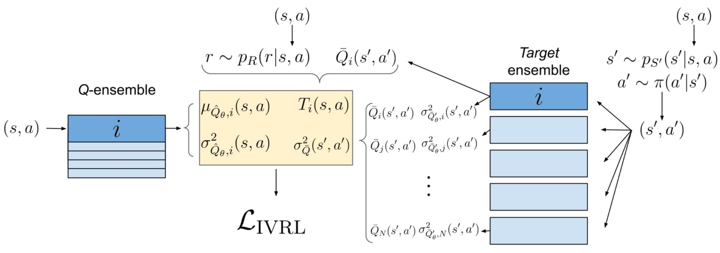
In most model-free deep reinforcement learning algorithms, such as DQN (Mnih et al., 2013) and SAC (Haarnoja et al., 2018), a policy \( π \) is evaluated at state-action pair (\(s,a\)). To learn how to evaluate the said policy, a neural function approximator is trained using the supervision of a target \( T \).
To obtain this target, the agent remembers:
- The reward \( r \) it received and;
- the state \( s’ \) it reached after taking action \( a \) at state \( s \).
- The agent then imagines what action \( a’ \) would be given by the policy at \( s’ \).
- It then uses its current (and imperfect) policy evaluation to obtain the Q-value at (\(s’,a’\)).
- The target \( T \) is then computed by: \(T(s,a)=r+\gamma \bar{Q}(s′,a′)\).
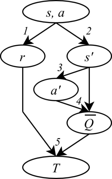
Steps 1, 2 and 3 can be stochastic, and step 4 is based on the current (and uncertain) estimation of the Q-value. These create noise on the labels of the supervision task: learning to predict the policy value. Such noisy supervision slows down the learning.
The key insight of the project is that the noise on the target is heteroscedastic, i.e. that it is not always sampled from the same distribution. If the variance of this distribution is known, it is possible to mitigate the effects of the noisy supervision by applying a weighting scheme that downweights high-variance samples, and thus to improve the sample efficiency of DRL algorithms.
The two main contributions of Inverse-Variance Reinforcement Learning (IV-RL) are thus the evaluation of the variance of the target distribution, and the use of the appropriate weighting scheme.
Evaluating the variance of the target
We evaluate the variance of the target from two ends. First, we use variance networks, trained using the negative log-likelihood (NLL) loss function.
\( L_{NLL}(x,y,\theta)=\frac{|f(x,\theta)-y|^2}{\sigma^2}+\ln(\sigma^2) \)
In supervised learning, the NLL loss leads the network to predict the variance of the labels for a given input. For example, if we have several labels for the same input \((s,a)\), the network’s prediction will tend towards \(\mu(s,a)\), the mean of the labels, and the network’s variance prediction will be the variance of these labels.
We use variance networks with NLL to estimate the variance in the target due to the stochasticity of steps 1, 2 and 3. For a better insight, assume for a moment that the value of \(\bar{Q}(s′,a′)\) used in the target is always the same given \((s’, a’)\). In that case, for a given \((s,a)\) pair, having different targets \(T\) will be due to getting different values of \(r\), \(s′\) and \(a′\). The variance output by NLL thus captures the effect on the target of the stochasticity of the reward (1), of the environment dynamics (2), and of the policy (3).
We also want to estimate the predictive uncertainty of \(\bar{Q}(s′,a′)\), which is bootstrapped in step 4. Due to lack of experience, this value is noisy. For example, at the beginning of the training process, the value estimator has no idea of the true value of \((s’,a’)\). Here, we used variance ensembles (Lakshmiranayanan et al., 2016): instead of a single variance network, we train 5 variance networks separately, with differences in the initial conditions and training sets. Each network predicts a mean and a variance for \(\bar{Q}(s′,a′)\). The variance of \(\bar{Q}(s′,a′)\) is then computed by computing the variance of the resulting mixture of Gaussians. The intuition here is that the networks will only converge in their predictions if they have been sufficiently trained on the surroundings of \((s’,a’)\). Otherwise, their predictions will diverge, producing a higher variance.
Weighting scheme and loss function
Once we have these two variance measures for a single target, how can we use them to mitigate the effect of the noise? In the case of heteroscedastic regression, when the variance is known, we can use weights in the loss function to reduce the impact of labels with high noise, while increasing trust in the labels with a low amount of noise. In the case of linear regression, the optimal weights are the inverse of the variance. It is harder to prove they are optimal in the case of neural networks optimization, but we can follow the same idea.
To account for the predictive uncertainty, we use a weighting scheme called Batch Inverse-Variance (BIV) (Mai et al., 2021). The inverse variance weights are normalized over the mini-batch and a hyperparameter allows to control the intensity of the weighting scheme through the effective batch size. This allows robustness, especially as the variance estimation methods we use do not always work smoothly: the variance can be strongly under or over estimated. Once again, we show that using only BIV with ensembles (without variance ensembles) improves the sample efficiency.
We combine both in a multi-objective loss function, leading to consistently better performances than when only considering one or the other uncertainty prediction.
Framework and existing work
We applied Inverse Variance RL (IV-RL) on DQN and SAC. This implementation requires a lot of design choices. In addition, ensembles can also be used for uncertainty-aware exploration strategies, which we used although they are not our contribution. We built our IV-RL framework upon existing works, in particular: BootstrapDQN (Osband et al., 2016), Randomized Prior Functions (Osband et al., 2018) and SUNRISE (Lee et al., 2020). Also note that UWAC (Wu et al., 2021) is a very interesting piece of work in the same direction as IV-RL, although looking at the slightly different problem of batch RL under the angle of out-of-distribution sample detection.
Results
IV-RL shows a significant improvement in the sample efficiency and the learning performance when applied on DQN and SAC, as shown in the figures below.


More results are available in the paper and the additional contents, including ablation studies, studies of the influence of some hyperparameters, variance estimation plots, and performance of other architectures and weighting schemes.
Significance and further work
In IV-RL, the Bellman update is seen under the angle of noisy and heteroscedastic regression. This leads to the challenges of estimating the target variance and using it to reduce the effect of noise. The significant improvements shown in the results prove that this angle of analysis is a direction which could help the field of DRL overcome the challenge of sample efficiency.
Implementing these insights is difficult. The variance estimation techniques used in IV-RL are tricky. They are subject to counter-intuitive learning dynamics and the scale of the predicted variances is not calibrated. To integrate them into the IV-RL algorithms, we had to take several steps to improve the robustness to over or under-estimated variance values – sometimes, having to tradeoff with weight discrimination power (using \(\xi\) in BIV) or computational efficiency (using ensembles).
In addition, due to the NLL formulation already using inverse-variance weights, the two estimated variances could not be added to each other in a single objective loss function, as would logically be the case following our theoretical analysis. This could be a direction for improvement of the algorithm. IV-RL proves that taking uncertainty of the target into account in the Bellman update is a highly promising direction to improve sample efficiency in DRL. It is a working, sample-efficient algorithm which can be used as is. It is also a proof of principle which could be improved: we strongly encourage further work in that direction, as well as in its adaptation to other DRL algorithms and subdomains.
Official publication: https://openreview.net/pdf?id=vrW3tvDfOJQ
ArXiv pre-print: https://arxiv.org/abs/2201.01666
Source code on Github: https://github.com/montrealrobotics/iv_rl
References
Volodymyr Mnih, Koray Kavukcuoglu, David Silver, Alex Graves, Ioannis Antonoglou, Daan Wierstra, and Martin Riedmiller. Playing Atari with deep reinforcement learning. NIPS, pp. 9, 2013.
Ian Osband, Charles Blundell, Alexander Pritzel, and Benjamin Van Roy. Deep exploration via bootstrapped DQN. arXiv:1602.04621, Jul 2016.
Ian Osband, John Aslanides, and Albin Cassirer. Randomized prior functions for deep reinforcement learning. In Advances in Neural Information Processing Systems, volume 31. Curran Associates, Inc., 2018
Tuomas Haarnoja, Aurick Zhou, Pieter Abbeel, and Sergey Levine. Soft actor-critic: Off-policy maximum entropy deep reinforcement learning with a stochastic actor. arXiv:1801.01290, 2018.
Kimin Lee, Michael Laskin, Aravind Srinivas, and Pieter Abbeel. SUNRISE: A simple unified framework for ensemble learning in deep reinforcement learning. arXiv:2007.04938, Jul 2020.
Yue Wu, Shuangfei Zhai, Nitish Srivastava, Joshua Susskind, Jian Zhang, Ruslan Salakhutdinov, and Hanlin Goh. Uncertainty weighted actor-critic for offline reinforcement learning. arXiv:2105.08140, May 2021.
Vincent Mai, Waleed Khamies, and Liam Paull. Batch inverse-variance weighting: Deep heteroscedastic regression. arXiv:2107.04497, Jul 2021.
