Learning Better Representations by Interpolating Hidden States

Deep neural networks are typically trained via empirical risk minimization, which optimizes a model to perform well on the data points observed during training. As a result, the trained network is very accurate on data points that are similar to those seen during training, but often performs poorly  on data points away from the training distribution (since its generalization behavior is only weakly constrained by the architecture).  

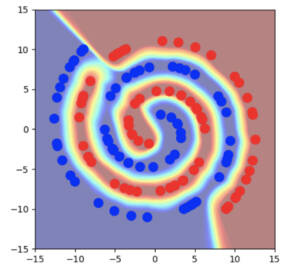
To see this more concretely, consider the simple case of training on 2D spirals with a limited number of labeled training samples.  We also use an architecture where one of the hidden layers has only two dimensions, so that we can directly visualize what is happening in the hidden states: 

Fig : A neural net trained to classify on two interlocked spirals.  The model’s classification decision in the observed space (left) and the decisions at different points in a 2D bottleneck hidden space (right) shows that  the normal training of neural networks leads to a decision boundary which is non-smooth and at very close to class boundaries at many places. 

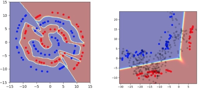
Even though this is a simple two-dimensional example, it illustrates several basic problems in the usual empirical risk minimization framework: 

• The model has very high confidence over almost all of the space, both in the input space and the hidden space (the red or blue regions indicate high confidence). 
• The decision boundary cuts very close to real data points. 
• The encoding of training points occupy a large volume in the hidden space.  

To help address these issues, we consider training on combinations of attributes from multiple examples. While this is still an active area of research, we propose a simple technique that we call Manifold Mixup: 

• We use a simple linear interpolation to combine the hidden states between pairs of examples. While this doesn’t consider all ways of combining information, there is evidence from the research on embeddings that linear combinations of hidden states can be semantically meaningful. 
• To label these combined points, we use the same linear combination of the targets for the selected example pairs (for the case of cross-entropy loss, this is equivalent to taking a weighted average of the losses). 
• Higher level layers are more abstract and thus might be better covered by simple linear interpolations.  On the other hand, they remove more of the details from the original data. To sidestep this tradeoff, we perform mixing on a random layer for each example.  

Memory and computation are important constraints for researchers and practitioners alike. Manifold Mixup requires virtually no additional computation or memory, since it only requires combining hidden states and class labels as an additional computation step and it does not have any additional memory requirement.

How does it work?

The procedure for manifold mixup can be described very simply, and only introduces two hyperparameters: alpha (the mixing rate) and S (the set of layers to consider mixing in): 

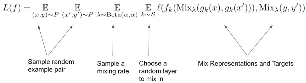
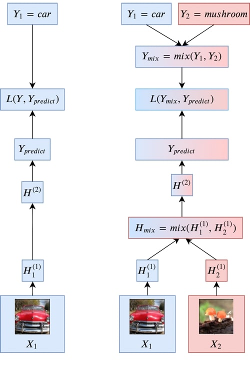
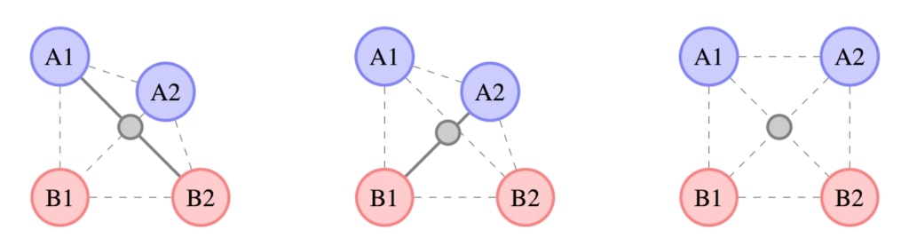
A more diagrammatic description of Manifold Mixup is given in the below figure.

Figure.  Left: The normal forward pass for training Deep Neural Networks. Right: The forward pass in the Manifold Mixup training. The gradient is back-propagated all the way down to the bottom-most layer in Manifold Mixup training.

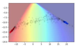
Going back to the spirals example, we can see that the decision boundary is placed much further away from the real data points, both in the input space and in the hidden space.  We also see a much larger region of uncertainty away from the real data points. However, one rather puzzling effect is that we can see that the hidden state values for real data points become very concentrated. In this example, they’re almost concentrated to a single point!  

Why do the hidden states get rearranged when training with Manifold Mixup? This property is not obvious at first, but is more apparent  if one considers what types of data will have the best fit under a linear model. Any direction which points between different classes should have no intra-class variability. Thus, the within-class variability and between-class variability are pushed onto orthogonal linear subspaces. In a binary classification problem with a 2D hidden space, this has the effect that each class gets pushed down to a single point.  

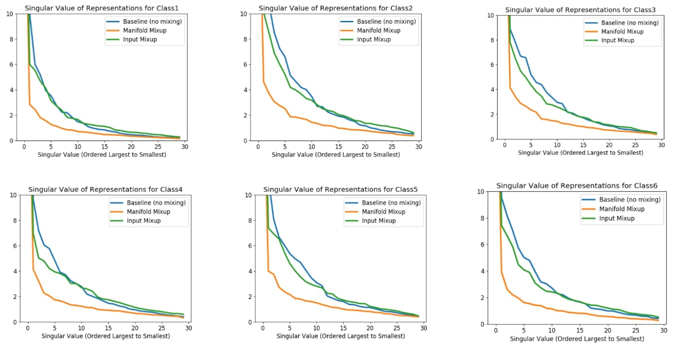
While we first observed this dramatic change from using Manifold Mixup on 2D toy problems, we became curious about whether this phenomenon also holds in higher dimensional spaces.  Moreover, what does this concentration effect even mean in a higher dimensional space?  

To explore the higher dimensional behavior empirically, we turned to the technique of singular value decomposition. This technique consists of fitting ellipses to a set of points in a (potentially high-dimensional space), and then studying how many dimensions of significant variability the ellipse has. The lengths of the axes of the ellipse are referred to as “singular values”. If all singular values are the same, it indicates that the data points roughly form a sphere. If only one singular value is large, it indicates that the data points roughly follow the shape of a narrow, tube-like ellipse.  In practice, we found that Manifold Mixup had a significant impact on this elliptical approximation of the hidden states. More specifically we found that using Manifold Mixup dramatically reduced the number of directions in hidden space with substantial variability.  

Figure: We observed the flattening effect from training with manifold mixup in problems with a higher-dimensional hidden state. Notably, we can see in higher dimensional spaces that the flattening effect is not so restrictive that each class gets pushed to a single point, rather each class is allowed to vary within a lower dimensional subspace.  

Results from Manifold Mixup

While manifold mixup has interesting properties, it also turns out to be a well-performing regularizer on real tasks. In particular, we have shown in this work that Manifold Mixup outperforms other competitive regularizers such as Dropout, CutOut and Mixup (See full paper for further details).

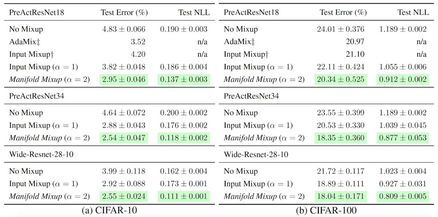
We also note that Manifold Mixup often dramatically improves likelihood on the test set, which we believe to be related to the model having lower certainty away from the training data’s distribution. This is critical for achieving good test likelihood, as confidently but incorrectly classified points can dramatically worsen test likelihood (in fact a single point could bring the likelihood to zero).  

Furthermore, we found that Manifold Mixup is very robust to its two hyperparameters: the choice of layers to perform mixing as well as the mixing rate (alpha).  

New Developments

Despite being relatively recent (ICML 2019), the Manifold Mixup technique has seen several exciting developments. Several applied research projects have successfully used Manifold Mixup. 

Bastien et al. (2019) demonstrate accuracy improvements in handwritten text recognition using manifold mixup.  One notable aspect of this work is that they used a structured loss, which was mixed between different examples, instead of directly mixing targets as we did in our Manifold Mixup work.  Mangla et al. (2019) combine Manifold Mixup with self-supervision strategies (such as rotation prediction) for achieving state-of-the-art results on the Few-shot Image classification task. Verma et al. (2019) propose to train fully-connected network with Manifold Mixup jointly with a graph neural networks for the node classification tasks, and have demonstrated substantial improvements in results including state-of-the-art results on several competitive datasets.  In terms of the theory of Manifold Mixup, Roth et al. (2020) have investigated flattening in the context of transfer learning.

This blog post is based on our paper:
Manifold Mixup: Better Representations by Interpolating Hidden States
Vikas Verma, Alex Lamb, Christopher Beckham, Amir Najafi, Ioannis Mitliagkas, Aaron Courville, David Lopez-Paz, Yoshua Bengio
ICML 2019 (https://arxiv.org/abs/1806.05236)

References:

[1] Moysset, Bastien, and Ronaldo Messina. “Manifold Mixup improves text recognition with CTC loss.” 2019 International Conference on Document Analysis and Recognition (ICDAR). IEEE, 2019.
[2]Mangla, Puneet, et al. “Charting the right manifold: Manifold mixup for few-shot learning.” The IEEE Winter Conference on Applications of Computer Vision. 2020.
[3] Verma, Vikas, et al. “Graphmix: Regularized training of graph neural networks for semi-supervised learning.” arXiv preprint arXiv:1909.11715 (2019).
[4] Roth, Karsten, et al. “Revisiting training strategies and generalization performance in deep metric learning.” arXiv preprint arXiv:2002.08473 (2020).